Magnetic Resonance Imaging (MRI)#
Further Reading
This page introduces MRI at a high level but is not intended to be a thorough treatment of the subject. For a more detailed treatment of neuroimaging and MRI, we recommend this course by David Heeger. For a deep dive into how MR measurements work, we suggest this online course by Marty Sereno. A YouTube playlist of the lectures can be found here.
There are many methods of noninvasively studying the human brain, but MRI is the method best suited to examine the organization of functional maps on the cortical surface. MR imaging is a method of measuring the chemical properties of a 3D region of space or of many small 3D regions. MRI machines take 3D images made up of voxels—3D pixels. The intensity measured at each voxel is related to its concentration of a particular kind of chemical property that depends on the kind of scan. There are many kinds of MRI scans, but for studying how the visual system is organized in the brain, we will focus on three of them: structural scans, diffusion-weighted scans, and functional scans.
Structural MR Imaging#
The most important kind of structural MR image is called a T1-weighted image. Precisely what T1-weighted images measure is beyond the scope of this document, but T1-weighted images are useful for imaging the brain because voxels tend to be bright when the concentration of fat is high and low when the concentration of water in the voxel is high. When a T1-weighted image is taken of the brain, the brain appears much brighter than the cerebrospinal fluid around it, making the voxels that are part of the brain easy to distinguish from the voxels that are not (Fig. 5). Additionally, the white matter voxels appear brighter than the gray matter voxels because white matter contains myelin, which has high fat content. Because of these contrasts, T1-weighted images are useful for determining the precise shape of the brain and in particular the white and gray matter, which have complex folded shapes.
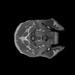
Figure 5. A T1-weighted image, rendered one slice at a time. The anatomical structures in the head and neck as well as the shape of the white and gray matter of the cerebral cortex are clear due to the contrast differences in the tissues.#
High resolution structural images such as T1-weighted images with voxels less than 1 cubic mm in size can typically be collected quite quickly, often just a few minutes.
Diffusion-weighted Imaging (DWI)#
DWI is a kind of structural MR imaging that measures the rate of diffusion of water in many directions in each voxel. These diffusion measurements can be used to reconstruct the shape and direction of white matter fiber tracts because water diffuses more readily along than against dense fiber tracts. For this reason, DWI is the state of the art noninvasive method to image the brain’s white matter structure.
Functional MR Imaging (fMRI)#
Functional MRI typically measures the blood oxygenation-level dependent (BOLD) signal, which measures the ration of oxygenated to deoxygenated hemoglobin in the blood of a voxel. Because neurons expend oxygen quickly when firing, additional oxygenated blood must flow into a voxel shortly following any substantial neural activity.
This BOLD signal can thus be used to deduce neural activity, albeit at the scale of voxels. Functional voxels are typically large than structural voxels—2 mm on each side or larger—and depending on their size contain on the order of 100,000–1 million neurons. In the visual system, voxels are characterized by their population receptive fields (pRFs). The name pRF comes from the observation that voxels contain populations of neurons combined with the concept of a neuron’s receptive field (RF). Neurons in the visual system are characterized by the region of the visual field in which a stimulus causes them to fire: their RF. A pRF is just a population of RFs. (See the chapter on pRFs for more information.)
FMRI images are usually taken at regular intervals of time in order to visualize the change in the BOLD signal. The timing of these signals is typically around 0.5–3 seconds, depending on the kind of experiment being run.